The Fraunhofer and Fresnel approximations

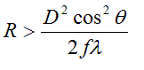
Our calculus of phase threads is a pretty general principle, but in practice, we often make certain approximations, which are referred to by different names.

Whenever all the phase threads are effectively parallel to one another, then we refer to the resulting diffraction pattern as a Fraunhofer, or Fourier domain, or far-field diffraction pattern. We've already discussed one type of Fraunhofer pattern with our Young's slits experiment. The diagram looked like this:

Well, the threads are not perfectly parallel here. But if we were to make the hemi-sphere very, very large, then all the threads would be parallel. The pattern we see would exist purely as a function of angle around the hemi-sphere. The co-ordinates of Frauhofer diffraction are therefore angles (or, more precisely, direction cosines). For all threads to be parallel, the object of interest (in the case above, the separation of the slits) must be small and the radius of the hemi-sphere must be large. How small and how large these dimensions are allowed to be depends on the wavelength, which determines the allowable error caused by the threads not being quite parallel.

We have an easy way of making a Fraunhofer diffraction pattern in the electron microscope. We just press the 'diffraction' button. Remember, we are imaging the back-focal plane, which by definition is where all parallel beams emerging from the specimen come to a focus:

On the contrary, Fresnel diffraction is the term used whenever we cannot make this 'parallel thread' approximation, in other words when we want to calculate a wave near a source of scattering.

Validity limits of the Fraunhofer approximation:

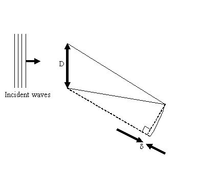
We can work out a rough expression for when the Fraunhofer condition applies by considering when the ‘parallel thread’ approximation breaks down. Two parallel threads subtending from opposite edges of the scattering object, of width D, at some angle, say θ, have a path length difference between them of p, as shown in the following diagram:

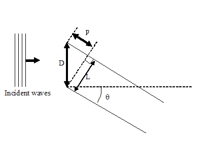
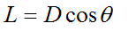
In this diagram, L = D cosθ (we will use this quantity below).

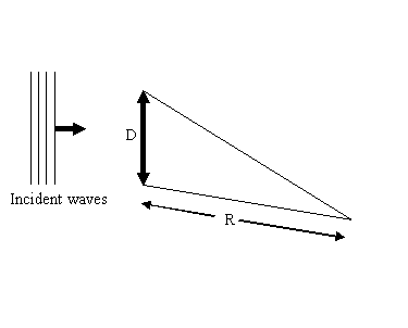
Now in the Fresnel condition, the threads meet up at a position relatively close to the scattering object, say at a distance R, like this:

If we suppose that the upper of the thread is at the same angle in the two diagrams, then what is the effect of the path length change of the lower thread being at a different angle in the two diagrams? Well, imagine holding onto the two threads, keeping the one upper stationary, we swing the lower thread upwards, like this:

We see that the lower thread describes an arc of a circle, and the extra path length added to it as a result of no longer being parallel with the upper thread is δ. If we remember our elementary geometry, then for any two chords of a circle PQ and ST crossing each other at O, like this

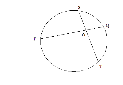
then the lengths PO times OQ equals SO times OT. In our case, we can redraw our two threads inscribed in a circle of radius R, like this:

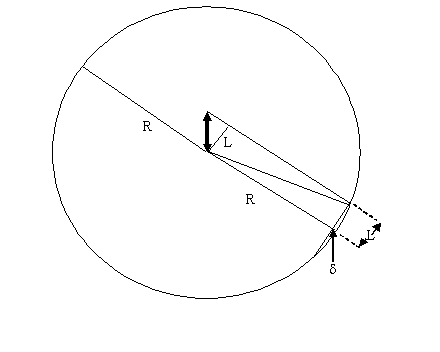
where L is as defined earlier. We see that (assuming 2R - δ is roughly 2R)

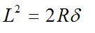
where

We generally wish to know how large R has to be in order for the Fraunhofer condition to apply. Clearly, this all depends upon how much of a phase error (caused by the non-parallel threads) we are prepared to tolerate. The phase error in radians is given by 2πδ/λ, where λ is the wavelength of our radiation. The total sum of adding up all the various complex values of our phase threads will be radically different if the contributions from the extreme edges of the scattering object are completely out of phase, that is if δ =λ/2. In practice, we probably want the error to be much less than λ/2, say fλ, where f is a small fraction. In this case, the Fraunhofer condition is satisfied if

In electron microscopy, the scattering angles are generally small (one to ten degrees), and so we can further approximate that L is about equal to D. So very roughly speaking, we reach the Fraunhofer condition when

Other important differences between Fraunhofer and Fresnel diffraction:

1) Movement:

We can formulate the definition of Fraunhofer diffraction from a completely different perspective: a Fraunhofer diffraction pattern does not move as the object (together with the illuminating radiation) is moved laterally.

Unless we use a lens to form the diffraction pattern, then if R (the distance to the recording plane) is very large, the diffraction pattern will not appear to move relative to the total size of the pattern itself. So for example, if we have an object which is 100nm in size, the electron wavelength is 0.0025nm, and the phase error we are prepared to tolerate in our phase threads is f =1/10 (a phase error of 36 degrees), then R must be larger than 200 microns. In any experimental set up, R would typically be of the order centimetres, and so the Fraunhofer condition is very well satisfied for this object size.

A typical electron diffraction pattern would extend up to about +/-10 degrees, and so when R = 200 microns, the total width of the pattern is about 40 microns. Now if we were to move the object laterally by its width (100nm), the diffraction pattern will also move by 100nm, but this is only 0.25% of its total width, and so we will not notice any substantial change in its position. When we use a lens to form the Fraunhofer pattern, even this tiny movement is eliminated (unless of course we moved the object so far that the diffracted beams miss the lens entirely! – in fact, for an aberrated electron lens, there will be a slight movement – but this is not important in the present context).

In summary, Fraunhofer patterns are fixed in position: they do not move as a function of shift of the scattering object. On the contrary, a Fresnel diffraction pattern (like the Fresnel fringes we discussed earlier) is recorded much closer to the scattering object: these patterns move in a way that directly corresponds with any shift in the object.

2) Propagation

The term ‘propagation’ in the context of waves means the act of allowing the wave to move forwards in space and time. Many wave patterns are stationary, in the sense that the pattern of intensity of the wave stays the same, even though the underlying wave continues to move constantly. Propagation is a mathematical way of finding out how the shape of the wave changes as it spreads from one region of space (usually in a plane, like the image plane or the diffraction pattern plane) to another. In electron microscopy we usually forget about time dependence, so propagation is just about finding out how the wave amplitude changes in space.

Another key difference between Fresnel and Fraunhofer diffraction is that Fresnel diffraction patterns change as we propagate them further ‘downstream’ of the source of scattering, whereas the shape of the intensity of a Fraunhofer diffraction pattern stays constant. In fact, as far as any real physical detector is concerned, as we move further and further away from the object, the Fraunhofer pattern gets bigger and bigger, and its intensity at any one point gets smaller (although the overall integrated intensity remains constant): however, its overall shape does not change. This is because the Fraunhofer pattern is a function of angle only. Once R is large enough to satisfy the Fraunhofer condition, the relative phase of the threads at any one angle do not change as R increases further.

On the contrary, a Fresnel diffraction pattern does change in shape as we move further away from the object (until, of course, we are so far away that the Fraunhofer condition is satisfied). It is easy to understand this in terms of phase threads. When we are close to an object of substantial size, the phase threads are extending towards us over a range of angles, like in the diagram we used earlier:

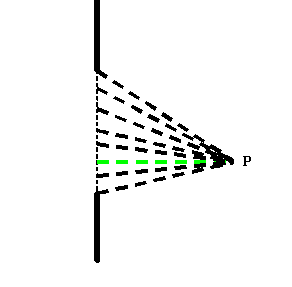
It is pretty clear that as we move the point P away from the object (hence we propagate the wave towards the right) then the relative lengths of the phase threads change with respect to one another. If the wavelength is short, even small changes in the relative length of the phase threads will radically affect the final result we obtain when we add up all the complex values corresponding to each thread.

In summary, near a source of scattering, the shape of wave changes substantially as we move away from the object. Eventually its shape settles into a Fraunhofer diffraction pattern (when R is large, given the size of the object and λ). From that point onwards, the shape of the wave intensity just physically expands as we move away even further, but its shape stays the same.

(Aside: If we form a Fraunhofer diffraction pattern using the back focal plane of a lens, then it is not true that if we move away from this plane – i.e. propagate the wave – that the pattern we observe remains the same. This is because of the way we are using the lens to bring what were parallel beams (threads) to a focus where they interfere. This focus occurs only at one very distinct plane, because the beams incident upon it are not parallel to one another, but are converging over a range of angles.)

3) The surface of calculation:

In the examples we’ve shown here, we have chosen to calculate Fresnel diffraction patterns on flat surfaces and Fraunhofer diffraction patterns on spherical surfaces. I think this is the logical way of approaching the subject, although it is not the way most textbooks derive the mathematics. The usual diagram is shown as follows:

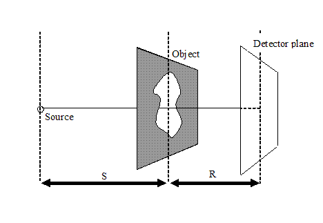
A source is position a distance S away from a flat surface, where some sort of aperture or object is positioned. A detector plane, also a flat surface, is positioned a distance R away on the other side of the aperture or object plane.

In our discussion above, we always assumed that the object was illuminated by a plane wave, which is equivalent to saying that S, the distance from the source to the object, is very large (in fact, the definition of ‘very large’ is the same as for R being large for the Fraunhofer condition to apply). As we move our detector plane from R=0 to R = large distance, then the pattern we record will start off as simply the intensity of the wave at the exit surface of the object function, it will then develop into a Fresnel pattern (complete with all the Fresnel fringes we discussed earlier, if there are sharp edges in the object), and then, as R is large enough to satisfy the Faunhofer condition, it will turn into a Fraunhofer pattern, from then on just getting larger and larger.

The trouble with this formulation is when we want to think about the phase of the underlying Fraunhofer diffraction pattern. Over a flat surface, the phase of the wave changes rapidly as we move away from the centre of the pattern, irrespective of whether we are in the Fraunhofer condition or not, as shown in the following diagram:

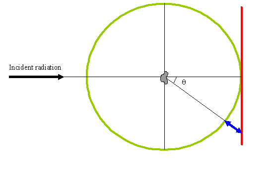
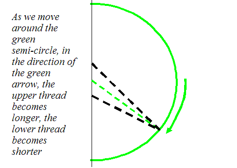
Here, the red line is a section through a flat detector plane, as in the conventional formulation. The green line is a section through a spherical surface, centred on the centre of the object function. We used the right of half green line in our discussion of Young’s slits.

The problem with the red line is that the underlying phase of the diffraction pattern over its length changes very rapidly as a function of θ, because of the extra path difference shown in blue. In fact, in the Fraunhofer condition, this extra path length difference (and hence phase change) has no bearing on the recorded intensity (except for a decay factor due to 1/R²), because all the contributing phase threads have the same path length (phase) added to them. The complex value of the wavefunction may vary very rapidly along the blue line, but its modulus (and hence intensity) remains constant.

Now, it is often said that the Fraunhofer diffraction pattern is the Fourier Transform of the exit wave coming out of the object function. In fact, the complex value of the wave over a flat surface (i.e. along the red line) is not the Fourier Transform of object exit wave. However, over the green line (a hemispherical surface) the complex value of the wave is mathematically equivalent to the Fourier Transform, at least for small values of θ.

In my experience, this little detail leads to all sorts of confusion.

First, it is sometimes said that validity of the Fraunhofer condition for the phase of the scattered wave is much more severe than for its intensity. That’s true if we insist upon talking about flat detectors (or flat planes on the entrance pupil of lenses that re-interfere the diffraction pattern) because of this extra path length. But in general it is much more natural to define the Fraunhofer pattern over a sphere, in which case this issue just doesn’t arise.

Secondly, because most the textbooks start off with a flat detector surface (which is, after all, not unreasonable), this extra ‘flat surface’ phase change is incorporated into the diffraction integral. Only by forming the intensity (which is often asserted quite early in the conventional derivation) is this extra phase obliterated (the wave is multiplied by its complex conjugate). However, this means that the direct connection between the mathematical device of the Fourier Transform and Fraunhofer diffraction plane is lost. Most texts undertake a change of coordinates (from the flat surface to angles of scatter) in order to bring out the equivalence. If we stick to the spherical surface (the green line) from the start, we don’t suffer any of these messy complications.

Another good reason for using the spherical surface is that (given appropriate scaling) it is equivalent to the Ewald sphere, an indispensable tool in all diffraction theory (that is, Fraunhofer diffraction theory) of the scattering of waves from three-dimensional objects. The green curve is then seen truly as a subset of a three- dimensional Fourier Transform of the object function, even at large values of θ (which in the diffraction literature is called 2θ_B, where θ_B is called the Bragg angle). This is even true for waves which have been scattered through an angle greater than 90 degrees.

Copyright J M Rodenburg