Fresnel fringes

At last, after all this pre-amble, we can get to talk about something we can really see everyday in the transmission electron microscope...

Experiment: Load a holey carbon film into the TEM - a standard carbon film test specimen with gold particles and graphite will also do, as long as it has got reasonably round holes in it. In fact, any specimen with sharp edges will do. Align the microscope as described in the alignment guide. Observe a small round hole in the carbon film and vary the objective lens defocus. At focus, the carbon is almost invisible. Either side of focus a bright or dark fringe appears near the edge of the carbon film. If you are using a microscope with a field-emission gun, then you might see several fringes, parallel to one another.

What's going on here? Well, as we change the focus of the objective lens, we change the height of the plane which we are imaging onto the phosphor screen. Ideally, we usually want this plane to be coincident with the specimen, but when we over-focus the objective, we are actually forming an image of a plane downstream of the carbon film, like this:

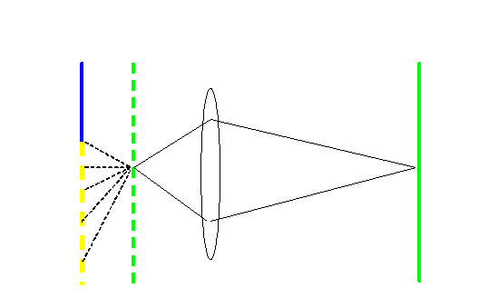
In this diagram, which is drawn at right-angles to the lenses in the alignment guide to be consistent with the earlier pictures in this section, the lens is over-focussed. It is imaging the dotted green plane onto the solid green image plane. The specimen (edge of the carbon film) is the blue line, and so it is out of focus. The yellow dotted line is free space, which we assume is illuminated by a plane wave. The dotted lines are our phase threads - that is, the lines of travel of little spherical waves, each one emanating from one part of the the yellow dotted line. We've only shown these meeting at a single point on the green dotted line.

It should be emphasised that the whole of the wave disturbance anywhere over the green dotted plane can be calculated by drawing together all the respective phase threads from the yellow dotted line. Indeed, the rays through the lens, which here we have drawn as solid lines, can themselves be thought of as phase threads, but we will do this later. (Remember: Huygen's Principle can be applied over and over again, from any surface of wave disturbance to any other surface of wave disturbance, whether it is an image, a diffraction pattern, or anything in-between. It is a very powerful concept.)

Now, the question is, what will our wave intensity look like in the image? In practice, the image is two-dimensional, but for a straight edge, we can just worry about plotting out the intensity across a line perpendicular to the edge, that is, across the green line in the diagram above. If we trust the lens works perfectly, then this is the same as calculating the intensity over the dotted green line.

It becomes clear that this integral (the summation or adding up of all the phase threads) is the same problem we discussed on the previous page. There, we qualitatively worked out the resultant wave vector at one particular point, P. How, do we work out the wave over the whole of the dotted line?

Think about it this way. If we removed the specimen entirely, the addition of all the phase threads would mean adding together in the complex plane the entire spiral of red wave vectors (see previous page). The resultant wave would have this amplitude, represented by the black vector:

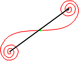
The complete spiral shown here is called Cornu's spiral. You can find it derived formally in any optics book. Now imagine slowly moving in the specimen, in other words, shifting the blue line downwards in the first diagram above. As it moves in, the specimen blocks off the spherical waves from one end of the spiral, removing these wave amplitudes from the integral. The spiral is slowly 'corroded' away, like this:

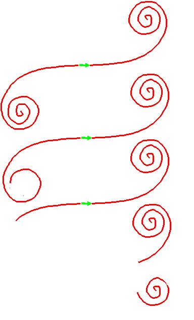
Of course, moving the specimen and calculating the image at one point is the same as keeping the specimen stationary, but calculating the image at different points relative to the edge of the specimen. As Cornu's spiral is corroded away, we are basically expressing how the wave changes across the green lines in the first diagram. So, to calculate the intensity of the image of a sharp, out-of-focus edge, all we to do is think how the resultant vector (actually, its length squared -its intensity) changes between the extreme ends of our partially corroded Cornu's spiral. To begin with, a long way from the specimen edge, the resultant will oscillate in length, because it goes round and round the bottom left bit of the spiral. Then it becomes quickly shorter. Finally, it slowly shrinks to nothing as the last of the top right part of the spiral disappears. Qualitatively, the intensity plotted across an edge looks like this:

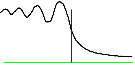
You can see these fringes - Fresnel fringes - occurring beside any edge in an out-of-focus electron image. Every time you see these things, you are proving to yourself that electrons behave as waves. As they pass a sharp edge, just like our water analogy with the harbour wall, the electron waves diffract. They 'slosh about' and make a standing wave interference pattern. If you have understood how we derived (entirely qualitatively, and without any formal mathematics) the above result, then you have really begun to understand wave interference.

Less important details:

In reality, our carbon film in our experiment does not stop or block off the incident plane waves. The waves actually pass through the film, but as they do so, they have a phase change induced upon them. However, it turns out that the qualitative behaviour of the resulting Fresnel integral is similar to what we describe above.

The exact form of the intensity depends on the wavelength of the electrons, the magnification of the lens, the amount of defocus, and the coherence of the illumination.

Copyright J M Rodenburg