The convolution integral

After the Fourier transform, the next most important mathematical idea in imaging and scattering theory is the convolution integral. When this is combined with the Fourier transform – via the ’convolution theorem’ – we have an extremely powerful method for understanding all sorts of optical and scattering phenomena: propagation, lens aberration theory, scattering theory, coherent convergent diffraction, multi-slice methods, the transfer function of CCD cameras and alike, and all sorts of other goodies. Indeed, many optical and diffraction textbooks include a great block mathematical relations concerning convolutions and Fourier transforms as ‘introductory concepts’ (often much to the mystification of the material and biological scientists).

Since these pages are intended for the less mathematically minded, I will approach convolution from what I hope is an intuitive point of view. However, we will have to use a few equations: these concepts are just so important that any serious electron microscopist or imaging scientist should understand the mathematical basics.

To start with, lets just think one of the very first diagrams we drew in the the beginner’s guide to TEM:

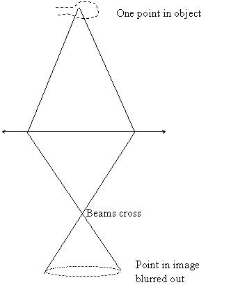
The idea of this picture was to show that when a lens is not focussed, a point that we are trying to image is blurred out into a circular patch. If two points near one another from the same object are out of focus, the blurred patches overlap and add together in the image plane, like this:

When we think of how all the points in the image add up in this blurring process, then what we are doing is forming a convolution.

So, one way of thinking of a convolution is to think of a picture, and then think how this is blurred out when the picture is out of focus. The out-of-focus image is the ‘true image’ blurred by a ‘blurring process’. We characterise the blurring process by a thing (the ‘blurring function’) which has the shape and structure of what would come out of blurring process if the ‘true image’ consisted of just a single point. This blurring function need not be symmetric (like the circle in the picture above), but can be any shape. For example, we know that astigmatism causes a streaking in the image: in this case, the image is a convolution of the true image with an oval shape.

Convolutions occur in many fields, and do not have to be about images: for example, spectroscopy often involves a one-dimensional convolution, similar to the what we describe below.

You can do a two-dimensional convolution experiment yourself with a magnifying lens. If you form an image of a distant object, like a street lamp at night, then a perfect lens would give a point (a dot) in the image plane. Now move the lens out of focus. You can make the blurring function very distorted by tilting the lens as well. If you now point the lens at an extended object (like an illuminated window if you are doing this at night), then you’ll see the convolution of the object with the blurring function. Similarly, people with bad eyesight see the image of world blurred out.

This ‘bluring process’ (a convolution) will be represented by the symbol. We’ll call the original image g, and we’ll call the blurring function h. The final blurred image we get we’ll call f. We can write the whole blurring process – the convolution – as:

Okay. Now all we have to do is work out what the convolution looks like mathematically, so we can work out how to actually calculate .

Unlike any conventional textbook, I want to describe two things, both of which are expressions of the convolution. The first is a physical description of how to make an experiment that performs an integration (an adding up of a signal) which is like the convolution integral. The second method, which relies on a slightly different view of convolution, is more the accurate mathematical description of it, but is harder to understand. Certainly, when I was first taught the convolution integral, the lecturer seemed to have some difficulty differentiating between this physical interpretation and the mathematical interpretation. I found it all very confusing. Perhaps this concern is peculiar to me. However, I do find that this is generally poorly explained in the textbooks, so here I am going to spell it out explicitly.

The physical detector integral:

My first version of the convolution integral I will call the ‘physical detector integral’. We’ll start just in one dimension: our two functions (the ‘true image’ and the ‘blurring function’ will each be one dimensional. This is what happens…

We have a distribution of radiation, say of light. This could be coming from any sort of optical instrument, like a spectrometer or diffractometer. The distribution is spread out across a surface, but only varies in one direction, like this:

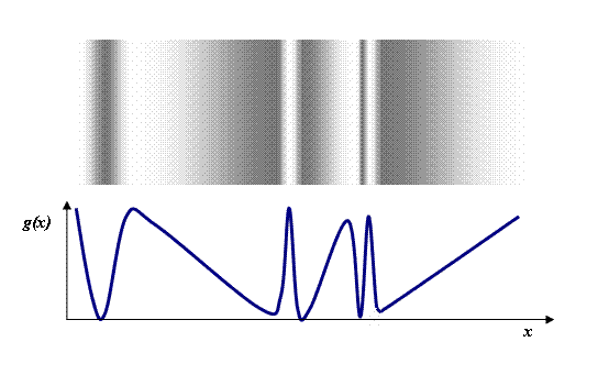
In this diagram, the top pattern is like the distribution of light cast upon a surface. The lower diagram is graph representing the intensity of the light, g(x), as a function of x, the distance measured horizontally across the surface.

Now supposing we want to record this distribution of light quantitatively. We could do this by letting the light distribution fall upon a photographic film. Alternatively, we could arrange for some sort of electronic light detector (e.g. a photodiode) to scan across the pattern. We could then read out the intensity measured by the detector as a function of its position: this process will perform a convolution.

Suppose a photo-detector is mounted behind a slit. Both the slit and the detector can be moved horizontally. The slit has a certain width which has the effect of adding up a region of the intensity pattern. It can be represented by a rectangular aperture superimposed upon the intensity pattern, like this:

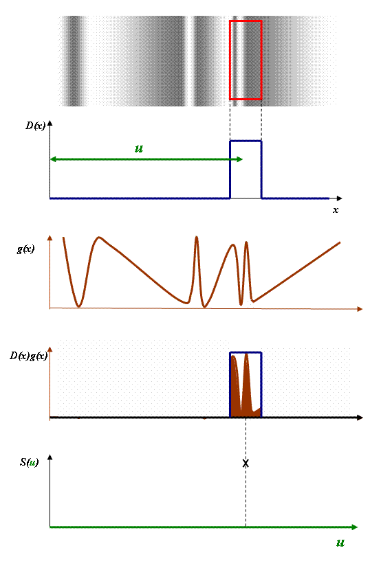
In the top-most plot, we have the physical intensity distribution with the shape of the slit superimposed upon it. Below it, we have a graphical representation of the sensitivity of the slit, a rectangular function, which we label D(x) (for ‘detector function’): here we assume that every part of the slit has equal sensitivity to the light. The centre of the slit is positioned a distance u away from the origin, shown in green.

In the next two plots in the diagram above, we have the original graphical representation of the intensity distribution of the light, g(x), and its product with D(x): i.e. g(x) times D(x) at every position, x. The total area of brown represents the total signal coming out of the detector. Because the slit has a substantial width, it integrates an area of the light distribution. Finally, this integral – the signal S(u) – is plotted at this particular position of the detector slit.

Now, as we increase u, the slit moves sideways, and we can plot each value of total signal coming out of the detector as a function of u. We can think of this plot as the convolution of g(x) with D(x). (In fact, it is not the precise mathematical definition of the convolution of g(x) with D(x), as we’ll see below, but it is a very good start.)

What will this convolution look like? Clearly, because the slit is quite big compared with some of the smallest intensity changes in the light distribution, the plot that we get out will be quite blurred compared with the original light distribution. g(x) will be ‘blurred out’ something like this:

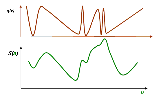
(This plot has been made by hand, and so is just qualitative.)

Now let’s try to write this down mathematically.

The first thing we need is a way of mathematically moving our slit function sideways. We can describe the slit function, D(x), as being centred on x=0, like this:

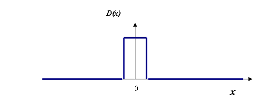
When the slit function is moved rightwards, say to a position where u (the amount of shift) is u=5, then what we need is D(x-5), where the function D is the same as it was before, but its co-ordinate is not ‘x’ but ‘x-5’. At first, it may be tempting to think that to move the slit in a positive direction we should add a positive ‘offset’ to the slit function, so that it becomes a function of ‘x+5’. However, thinking about it, when x=5, we want the value of the shifted slit function to be the same as it was when x=0 before it was shifted. When x=5, we achieve this because D(x-5)=D(0), so the graph of D(x-5) looks like this:

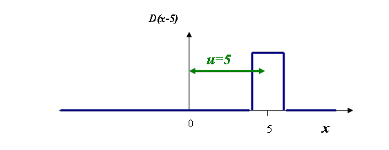
Of course, this argument is true for all values of u, so that means that the slit function shifted by any value of u is just D(x-u).

Coming back to our light detector, the signal out of the detector at any shifted position of the slit is just ‘the total added up detected light of g(x) times D(x-u)’. Or, in an equation,

Now this looks very much like the convolution integral, but it’s not quite right. According to the definitions we’ve used in this section, it does give the right answer for what comes out of our physical detector when it is moved a physical distance across a field of radiation. But this is not the mathematical definition (or, indeed, the most useful physical definition) of the convolution.

Convolution: the addition of impulse functions

The correct definition of a convolution is as an ‘addition of impulse functions’. An ‘impulse function’, or ‘impulse response function’, is the graph we would get out of our ‘physical detector integral’ if the light distribution (or whatever is represented by g(x)) is just a spike of intensity. This spike is technically called a delta function. It is related to the light distribution as follows:

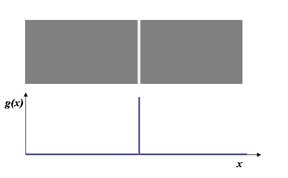
In other words, the distribution of light has zero intensity everywhere, except at one point along the x-direction, where there is a very bright peak. Ideally, this peak should be infinitesimally thin and infinitely high, but we’ll leave the exact mathematical definition until later.

Now, the convolution of our original detector function (a square top hat) with this spike is, pretty obviously, the shape of detector function itself. As a function of u, the displacement of our detector function that we described above, the convolution integral as we defined in the previous section looks like this:

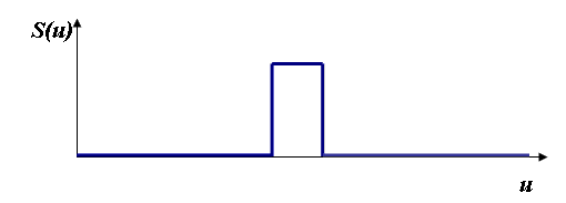
If you think about it, the integral of the D(x) times g(x) (which is now just a spike) is zero everywhere except where the spike of light intensity falls within the aperture of our detector. We measure a high intensity only for those values of u (the amount the detector has been shifted rightwards) where the light falls upon the detector.

Let’s now think what happens if our detector does not have the same sensitivity over the entire slit. So, for example, the detector function might instead look like this:

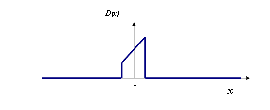
Here, the detector is physically more sensitive to light on its right-hand side than on its left-hand side.

Now what happens when we scan this uneven detector across a narrow spike of light? Well, as we begin to move the detector to the right, the spike of light is lying well to its right, and so we detect nothing, as before. As it moves further, the first bit of detector to hit the light beam is the most sensitive part of the detector (the extreme right-hand part of D(x)), so we suddenly get a big signal. As we move it further and further to the right, the less sensitive part of the detector is hit by the light, and so the signal gets smaller and smaller until it suddenly disappears when the detector moves out of the light entirely. So this is what S(u) will look like:

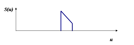
It would seem that the process of performing a convolution over a spike function (a delta function) has a given us a function that looks like D(x) flipped the wrong way round relative to the coordinate u.

This flipped around function is the definition of the ‘impulse response function’ of our detector: it is the signal that comes out of our system when an ‘impulse’ – that is the spike or delta function of light – is put into the experiment.

There are two important things to understand:

1) The convolution is always written in terms of impulse response functions, not the detector function that we thought about in the previous section. That is to say, when we write

then h(x) is the flipped detector function D(-x), not D(x), as we derived in the section above.

2) When we actually want to calculate the convolution integral, the way we can do it is indeed by thinking of the physical detector integral. But if we want to write this integral in terms of h(x), we must remember that h(x) = D(-x).

We decided in previous section that the physical detector integral was written

So now, in view of the second rule above, the proper definition of the convolution integral is

Note that the coordinates of the second term in the integral have been made negative relative to our first definition: this to account for the flipping effect. I think these negative coordinates are the most confusing aspect of the convolution, because if we think of physical detectors, the convolution really should seem to be written the other way round.

We also have another confusing problem in that we want the final answer to equal f(x) but we have already used x inside the integral. The more usual convention is to change the nomenclature inside the integral so that u=x (so that f(x) equals what we have previously called S(u)), and then we invent a new variable name for the existing x, say X. (X is sometime called a ‘dummy variable’, because once the integral has been performed, it disappears, and so we could call it anything we like: it does not affect the final answer.)

We end up with the formal definition of the convolution:

Remember: The convolution integral is written in terms of impulse response functions. An impulse response function is the result we get out of the convolution when the other function involved in the convolution is a delta function or spike. This statement is true for both g(x) and h(x).

Clearly, if h(x) was a delta function, which we’ll denote as δ(x), then the slit in our ‘physical detector integral’ is infinitesimally thin, but infinitely sensitive. As a consequence, the experiment of scanning the slit across g(x) reproduces g(x) perfectly – there is no blurring effect. So that means that

Similarly, if g(x) is a delta function, then

For these equations to be true, the convolution integral must be defined as taking one the functions and multiplying it by a flipped version of the other function displaced by a certain distance, and then integrating the product of these two functions for all values of the relative displacement of the two functions.

We can see that the delta function is to the convolution like unity is to normal multiplication. If we multiply a number by one, the result is that same number. The convolution of any function with the delta function is the original function. Like normal multiplication, the convolution in also commutative: g(x)h(x) = h(x)g(x).

Although we could define convolutions in terms of the ‘physical detector integral’ (that is, the relationship we developed for S(u) involving g(x) and D(x)) these neat relationships would no longer apply. So, although the physical detector integral is a very good analogy of the convolution, and indeed is a prime example of its experimental significance, it can be misleading. Just remember that the impulse response function arising from a physical detector is the shape of the sensitivity of the physical detector reversed (or ‘flipped’).

We can think of convolution in terms of impulse response functions alone as follows. Imagine one of the functions involved as being made up of millions of little ‘spike’ functions, each one of which has the value and height of the underlying function. So we could express the light distribution we used the example above like this:

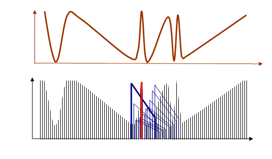
We know that any one spike gives an impulse response function of h(x). We now put an h(x) function scaled by the height of each spike at the position of that spike. At any one point, many of these h(x) functions will overlap. If we add up the value of all the overlapping h(x) functions at each point, then that is the value of the convolution at that point.

I’ve tried to draw this process (rather unsuccessfully) in the diagram above. I assume the impulse response function h(x) is the blue shape. The height of the thick blue function is scaled by the height of the red line. The thinner blue functions to its right are scaled by the respective heights of each of the spikes to the right of the red spike. At any one particular point, we have to add up all the blue functions that have a value at that point in order to calculate the convolution at that point. It’s perhaps not obvious that this gives the same answer as the ‘physical detector integral’ – but it does, as long as we remember that h(x) = D(-x).

Some final notes about convolutions

1) The examples we’ve given in this page involve only positive functions. That’s because we chose an example of measuring the intensity of light. In fact, in general, the functions f(x), g(x) and h(x) can all have negative or complex values: in coherent imaging theory, the functions are always complex, because they represent complex wave disturbances. The outcome of a convolution is then somewhat less obvious.

2) When h(x) or g(x) has negative or complex regions, then it’s not always true that a convolution ‘blurs out’ an image. In fact, it can have the effect of sharpening the image. Indeed, for every ‘blurring function’, h(x), convolved with an image g(x) to give f(x), there is an inverse function, say h’(x), which, when convolved with f(x), recovers g(x). This reverse convolution, called a deconvolution, is not always very well behaved – but that’s another story.

3) We can extend the concept of a convolution to any number of dimensions. In two dimensions (over image coordinates x and y) then:

4) Convolutions only work when the underlying dynamic of the image or signal formation process is linear. For normal wave propagation and interference, linearity is conditional on the linearity of the wave equation. In the case of electrons, linearity is guaranteed by virtue of the linearity of Schroedinger’s equation.

5) In imaging theory, it is not necessarily the case that the impulse response function of a lens (or, say, a spectrometer) is the same at all points across the image or spectrum. In this case, we cannot use the convolution theorem. In electron microscopy, the impulse response function is usually constant over the sort of fields of view we are usually interested in.

6) It is worth mentioning that the convolution integral can be used to solve inhomogeneous linear differential equations with boundary conditions, provided we can calculate the effect of an ‘impulse’ on the system. A general solution is then a super-position of all such impulses that make up a general input signal – in other words, a convolution. This is the fundamental idea behind Green’s function solution methods. An example of such a method in electron microscopy is Huygen’s principle.

Last posting 19/04/06: I add to these pages as I find time [recent update history]. I plan that the next posting will derive the convolution theorem and explore its applications in electron microscopy.

Copyright J M Rodenburg